Modeling
PyGrad offers an intuitive interface for building and training neural networks. Specifically, ANN-related components live in the pygrad.nn module. For those who are already familiar with PyTorch will immediately see that PyGrad’s API is no different from that of PyTorch. We hope to add more flavor to PyGrad’s API in the days to come.
Model Initialization
Below is a simple example of how to declare a neural network in PyGrad.
from pygrad import nn
from pygrad import functions as F

class NeuralNet(nn.Module):
    def __init__(
        self, num_input, num_hidden, num_class, dropout
    ):
        super(NeuralNet, self).__init__()
        self.fc1 = nn.Linear(num_input, num_hidden)
        self.fc2 = nn.Linear(num_hidden, num_class)
        self.dropout = nn.Dropout(dropout)

    def forward(self, x):
        x = self.fc1(x)
        x = F.relu(x)
        x = self.fc2(x)
        x = self.dropout(x)
        return x
pygrad.nn includes layers and the Module class through which neural networks can be initialized. Also noteworthy is pygrad.functions, which includes activation functions, trigonometric functions, as well as a host of other basic functions operations, such as reshape and transpose.
Saving and Loading Models
PyGrad offers an easy way of saving and loading model weights.
PATH = "my/model/save/path/filename.npy"

# save model
model.save(PATH)

# load model
model.load(PATH)
If the specified PATH is not appended with the .npy file extension, it will be added automatically. Note that save() will create a .npy NumPy binary save file that stores the model weights in the specified PATH.
Under the hood, PyGrad builds a weight_dict which is then serialized via NumPy’s binary file save and load backend. When loading the model weights, PyGrad calls model.load_weight_dict(). To see the weight_dictthat is created and loaded under the hood, simply call model.weight_dict().
>>> model.weight_dict()
{'fc2': {'W': array([[-0.0102793 , -0.43645453],
         [-0.5613075 , -0.40495454],
         [-2.06899522,  0.37147184],
         [ 2.74661644,  0.01093937],
         [ 1.43978999,  2.94304868],
         [ 0.11040433, -0.43386061],
         [ 0.31942078,  0.11889225],
         [ 2.18743003,  0.50037902],
         [-0.52810431, -0.11654514],
         [ 1.23020603,  1.06316066]]),
  'b': array([-0.19479341,  0.07610959])},
 'dropout': {'dropout': array(0.5)},
 'fc1': {'W': array([[ 0.21692255, -0.50617893, -1.36799705, -1.11569594, -0.25307236,
           0.60018887,  1.36053799, -0.63192337,  2.06461438,  0.5593571 ],
         [ 0.8679015 ,  1.1622997 ,  0.40791915,  0.90237478, -0.09208171,
           0.55416128,  0.52464201, -0.04155436, -0.23106663,  0.00484401]]),
  'b': array([-0.0241028 , -0.00574922, -0.14536121,  0.05873388, -0.20492597,
         -0.17550233, -0.16079421, -0.0762437 ,  0.05676356, -0.03754628])}}
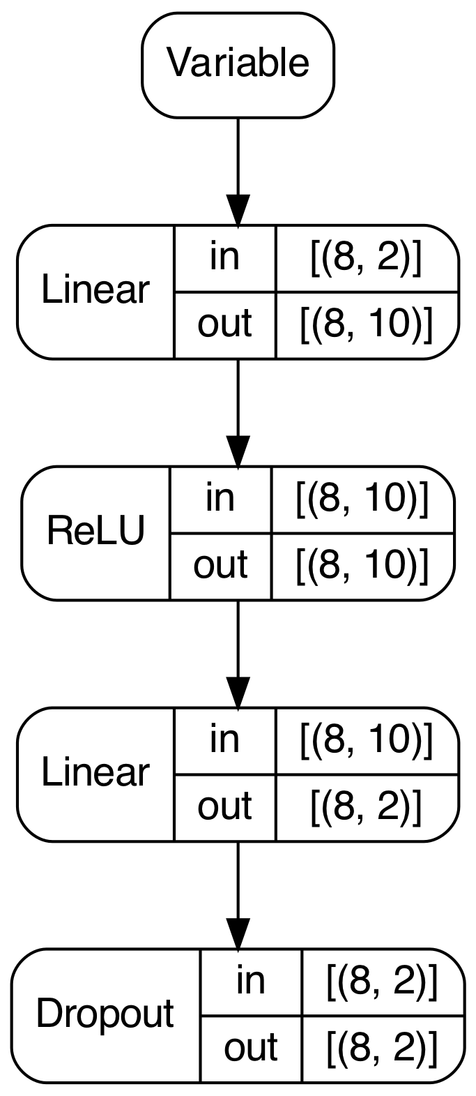
Model Visualization
PyGrad also provides useful model visualization using Graphviz. After a forward pass, PyGrad can traverse the computation graph to draw a summary of network’s structure, as well as the shape of the input and output for each layer.
model.plot()
In this instance, calling plot() on the model yields the following image.